Toy Regression

Run in Google Colab

View on GitHub

You will find here the application of DA methods from the ADAPT package on a simple one dimensional DA regression problem.

First we import packages needed in the following. We will use matplotlib Animation tools in order to get a visual understanding of the selected methods:

import numpy as np
import matplotlib.pyplot as plt
import matplotlib.animation as animation
from matplotlib import rc
rc('animation', html='jshtml')

Experimental Setup

We now set the synthetic regression DA problem using the make_regression_da function from adapt.utils.

from adapt.utils import make_regression_da

Xs, ys, Xt, yt = make_regression_da()
tgt_index_lab_ = np.random.choice(100,3)
Xt_lab = Xt[tgt_index_lab_]; yt_lab = yt[tgt_index_lab_]

We define here a show function which we will use in the following to visualize the algorithms performances on the toy problem.

def show(ax, y_pred=None, X_src=Xs, weights_src=50, weights_tgt=100):
    ax.scatter(X_src, ys, s=weights_src, label="source", edgecolor="black")
    ax.scatter(Xt, yt, s=50, alpha=0.5, label="target", edgecolor="black")
    ax.scatter(Xt_lab, yt_lab, s=weights_tgt,
                c="black", marker="s", alpha=0.7, label="target labeled")
    if y_pred is not None:
        ax.plot(np.linspace(-0.7, 0.6, 100), y_pred, c="red", lw=3, label="predictions")
        index_ = np.abs(Xt - np.linspace(-0.7, 0.6, 100)).argmin(1)
        score = np.mean(np.abs(yt - y_pred[index_]))
        score = " -- Tgt MAE = %.2f"%score
    else:
        score = ""
    ax.set_xlim((-0.7,0.6))
    ax.set_ylim((-1.3, 2.2))
    ax.legend(fontsize=16)
    ax.set_xlabel("X", fontsize=16)
    ax.set_ylabel("y = f(X)", fontsize=16)
    ax.set_title("Toy regression DA issue"+score, fontsize=18)
    return ax

fig, ax = plt.subplots(1, 1, figsize=(8, 5))
show(ax=ax)
plt.show()

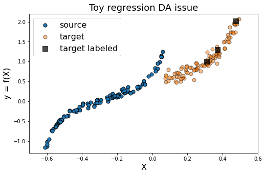
As we can see in the figure above (plotting the output data y with respect to the inputs X), source and target data define two distinct domains. We have modeled here a classical supervised DA issue where the goal is to build a good model on orange data knowing only the labels (y) of the blue and black points.

We now define the base model used to learn the task. We use here a neural network with two hidden layer. We also define a SavePrediction callback in order to save the prediction of the neural network at each epoch.

import tensorflow as tf
from tensorflow.keras import Sequential
from tensorflow.keras.layers import Input, Dense, Reshape
from tensorflow.keras.optimizers import Adam

def get_model():
    model = Sequential()
    model.add(Dense(100, activation='elu', input_shape=(1,)))
    model.add(Dense(100, activation='relu'))
    model.add(Dense(1))
    model.compile(optimizer=Adam(0.01), loss='mean_squared_error')
    return model

from tensorflow.keras.callbacks import Callback

class SavePrediction(Callback):
    """
    Callbacks which stores predicted
    labels in history at each epoch.
    """
    def __init__(self):
        self.X = np.linspace(-0.7, 0.6, 100).reshape(-1, 1)
        self.custom_history_ = []
        super().__init__()

    def on_epoch_end(self, batch, logs={}):
        """Applied at the end of each epoch"""
        predictions = self.model.predict_on_batch(self.X).ravel()
        self.custom_history_.append(predictions)

TGT Only

First, let’s fit a network only on the three labeled target data. As we could have guessed, this is not sufficient to build an efficient model on the whole target domain.

np.random.seed(0)
tf.random.set_seed(0)

model = get_model()
save_preds = SavePrediction()
model.fit(Xt_lab, yt_lab, callbacks=[save_preds], epochs=100, batch_size=64, verbose=0);

def animate(i, *fargs):
    ax.clear()
    y_pred = save_preds.custom_history_[i].ravel()
    if len(fargs)<1:
        show(ax, y_pred)
    else:
        show(ax, y_pred, **fargs[0])

fig, ax = plt.subplots(1, 1, figsize=(8, 5))
ani = animation.FuncAnimation(fig, animate, frames=100, interval=60, blit=False, repeat=True)

ani

Src Only

We would like to use the large amount of labeled source data to improve the training of the neural network on the target domain. However, as we can see on the figure below, using only the source dataset fails to provide an efficient model.

np.random.seed(0)
tf.random.set_seed(0)

model = get_model()
save_preds = SavePrediction()
model.fit(Xs, ys, callbacks=[save_preds], epochs=100, batch_size=100, verbose=0);

fig, ax = plt.subplots(1, 1, figsize=(8, 5))
ani = animation.FuncAnimation(fig, animate, frames=100, blit=False, repeat=True)

ani

All

Same thing happen when using both source and target labeled data. As the source sample ovewhelms the target one, the model is not fitted enough on the target domain.

np.random.seed(0)
tf.random.set_seed(0)

model = get_model()
save_preds = SavePrediction()
model.fit(np.concatenate((Xs, Xt_lab)),
          np.concatenate((ys, yt_lab)),
          callbacks=[save_preds],
          epochs=100, batch_size=110, verbose=0);

fig, ax = plt.subplots(1, 1, figsize=(8, 5))
ani = animation.FuncAnimation(fig, animate, frames=100, blit=False, repeat=True)

ani

CORAL

Let’s now consider the domain adaptation method CORAL This “two-stage” method first perfroms a feature alignment on source data and then fit an estimator on the new feature space.

from adapt.feature_based import CORAL

save_preds = SavePrediction()
model = CORAL(get_model(), lambda_=1e-3, random_state=0)
model.fit(Xs.reshape(-1, 1), ys, Xt,
          callbacks=[save_preds], epochs=100, batch_size=110, verbose=0);

Fit transform...
Previous covariance difference: 0.024858
New covariance difference: 0.000624
Fit Estimator...

fig, ax = plt.subplots(1, 1, figsize=(8, 5))
X_transformed = model.transform(Xs.reshape(-1, 1), domain="src").ravel()
ani = animation.FuncAnimation(fig, animate, frames=100, blit=False, repeat=True,
                              fargs=(dict(X_src=X_transformed),))

ani

As we can see. when using CORAL method, source input data are translated closer to target data. However, for this example, this is not enough to obtain a good model on the target domain.

TrAdaBoostR2

We now consider an instance-based method: TrAdaBoostR2. This method consists in a reverse boosting algorithm decreasing the weights of source data poorly predicted at each boosting iteraton.

from adapt.instance_based import TrAdaBoostR2

model = TrAdaBoostR2(get_model(), n_estimators=30, random_state=0)

save_preds = SavePrediction()
model.fit(Xs.reshape(-1, 1), ys.reshape(-1, 1), Xt_lab.reshape(-1, 1), yt_lab.reshape(-1, 1),
          callbacks=[save_preds], epochs=100, batch_size=110, verbose=0);

Iteration 0 - Error: 0.5000
Iteration 1 - Error: 0.5000
Iteration 2 - Error: 0.5000
Iteration 3 - Error: 0.5000
Iteration 4 - Error: 0.5000
Iteration 5 - Error: 0.5000
Iteration 6 - Error: 0.5000
Iteration 7 - Error: 0.5000
Iteration 8 - Error: 0.5000
Iteration 9 - Error: 0.5000
Iteration 10 - Error: 0.5000
Iteration 11 - Error: 0.4864
Iteration 12 - Error: 0.4768
Iteration 13 - Error: 0.4701
Iteration 14 - Error: 0.4296
Iteration 15 - Error: 0.3781
Iteration 16 - Error: 0.3584
Iteration 17 - Error: 0.3212
Iteration 18 - Error: 0.2908
Iteration 19 - Error: 0.2293
Iteration 20 - Error: 0.1284
Iteration 21 - Error: 0.0371
Iteration 22 - Error: 0.0335
Iteration 23 - Error: 0.0259
Iteration 24 - Error: 0.0281
Iteration 25 - Error: 0.0275
Iteration 26 - Error: 0.0230
Iteration 27 - Error: 0.0200
Iteration 28 - Error: 0.0167
Iteration 29 - Error: 0.0191

def animate_tradaboost(i):
    ax.clear()
    i *= 10
    j = int(i / 100)
    y_pred = save_preds.custom_history_[i].ravel()
    weights_src = 10000 * model.sample_weights_src_[j]
    weights_tgt = 10000 * model.sample_weights_tgt_[j]
    show(ax, y_pred, weights_src=weights_src, weights_tgt=weights_tgt)

fig, ax = plt.subplots(1, 1, figsize=(8, 5))
ani = animation.FuncAnimation(fig, animate_tradaboost, frames=299, interval=120, blit=False, repeat=True)

ani

ani.save('tradaboost.gif', writer="imagemagick")

As we can see on the figure above, TrAdaBoostR2 perfroms very well on this toy DA issue! The importance weights are described by the size of data points. We observe that the weights of source instances close to 0 are decreased as the weights of target instances increase. This source instances indeed misleaded the fitting of the network on the target domain. Decreasing their weights helps then a lot to obtain a good target model.

RegularTransferNN

Finally, we consider here the paremeter-based method RegularTransferNN. This method fits the target labeled data with a regularized loss. During training, the mean squared error on target data is regularized with the euclidean distance between the target model parameters and the ones of a pre-trained source model.

from adapt.parameter_based import RegularTransferNN

np.random.seed(0)
tf.random.set_seed(0)

save_preds = SavePrediction()
model_0 = get_model()
model_0.fit(Xs.reshape(-1, 1), ys, callbacks=[save_preds], epochs=100, batch_size=110, verbose=0);
model = RegularTransferNN(model_0, lambdas=1.0, random_state=0)
model.fit(Xt_lab, yt_lab, callbacks=[save_preds], epochs=100, batch_size=110, verbose=0);

fig, ax = plt.subplots(1, 1, figsize=(8, 5))
ani = animation.FuncAnimation(fig, animate, frames=200, interval=60, blit=False, repeat=True)

ani