Sample Bias 2D

Run in Google Colab

View on GitHub

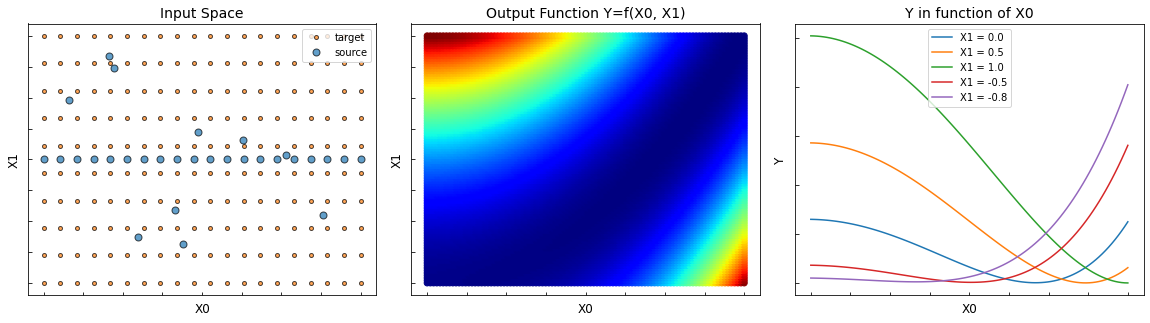
The following example is a 2D regression domain adaptation issue. The goal is to learn the regression task on the target data (orange points) knowing only the labels on the source data (blue points).

In this example, there is a sample bias between the source and target datasets. The sources are mostly located in X1=0 whereas the targets are uniformly distributed.

The following methods are being tested:

• Source Only

• KMM

• KLIEP

import numpy as np
import matplotlib.pyplot as plt
from mpl_toolkits.mplot3d import Axes3D
import matplotlib.animation as animation
from sklearn.neural_network import MLPRegressor
from sklearn.metrics import mean_absolute_error, mean_squared_error
from sklearn.metrics.pairwise import rbf_kernel
from adapt.instance_based import KMM, KLIEP

import tensorflow as tf
from tensorflow.keras import Sequential
from tensorflow.keras.optimizers import Adam
from tensorflow.keras.layers import Dense
from tensorflow.keras.models import clone_model

Setup

def f(x0, x1):
    x0 = (x0 + 1.) / 2.
    x1 = (x1 + 1.) / 2.
    return (1/100) * (100 * (x1 - x0**2)**2 + (1 - x0)**2)

np.random.seed(5)
Xs = np.stack([np.linspace(-1, 1, 20), np.zeros(20)], -1)
Xs = np.concatenate((Xs, np.random.random((10, 2)) * 2 -1))

xt_grid, yt_grid = np.meshgrid(np.linspace(-1, 1., 20),
                             np.linspace(-1, 1., 10))
Xt = np.stack([xt_grid.ravel(), yt_grid.ravel()], -1)

x_grid, y_grid = np.meshgrid(np.linspace(-1, 1., 100),
                             np.linspace(-1, 1., 100))
ys = f(Xs[:, 0], Xs[:, 1])
yt = f(Xt[:, 0], Xt[:, 1])
z_grid = f(x_grid.ravel(), y_grid.ravel())

fig = plt.figure(figsize=(20, 5))

ax1 = fig.add_subplot(1, 3, 1)
ax1.plot(Xt[:, 0], Xt[:, 1], '.', c="C1", label="target", ms=8, alpha=0.7, markeredgecolor="black")
ax1.plot(Xs[:, 0], Xs[:, 1], '.', c="C0", label="source", ms=14, alpha=0.7, markeredgecolor="black")
ax1.set_yticklabels([])
ax1.set_xticklabels([])
ax1.tick_params(direction ='in')
ax1.legend()
ax1.set_xlabel("X0", fontsize=12)
ax1.set_ylabel("X1", fontsize=12)
ax1.set_title("Input Space", fontsize=14)

ax2 = fig.add_subplot(1, 3, 2)
ax2.scatter(x_grid.ravel(), y_grid.ravel(), c=z_grid, cmap="jet")
ax2.set_yticklabels([])
ax2.set_xticklabels([])
ax2.tick_params(direction ='in')
ax2.set_xlabel("X0", fontsize=12)
ax2.set_ylabel("X1", fontsize=12)
ax2.set_title("Output Function Y=f(X0, X1)", fontsize=14)

ax3 = fig.add_subplot(1, 3, 3)
for x1 in [0., 0.5, 1., -0.5, -0.8]:
    X_ = np.concatenate((
        np.linspace(-1, 1, 100).reshape(-1, 1),
        np.ones((100, 1)) * x1), axis=1)
    ax3.plot(X_[:, 0], f(X_[:, 0], X_[:, 1]), label="X1 = %.1f"%x1)

ax3.set_yticklabels([])
ax3.set_xticklabels([])
ax3.tick_params(direction ='in')
ax3.legend()
ax3.set_xlabel("X0", fontsize=12)
ax3.set_ylabel("Y", fontsize=12)
ax3.set_title("Y in function of X0", fontsize=14)

plt.subplots_adjust(wspace=0.1)

Estimator

np.random.seed(0)
tf.random.set_seed(0)
model = Sequential()
model.add(Dense(100, activation="relu", input_shape=(2,)))
model.add(Dense(100, activation="relu"))
model.add(Dense(1, activation=None))
model.compile(loss="mse", optimizer=Adam(0.001))

fit_params = dict(epochs=300, batch_size=34, verbose=0)

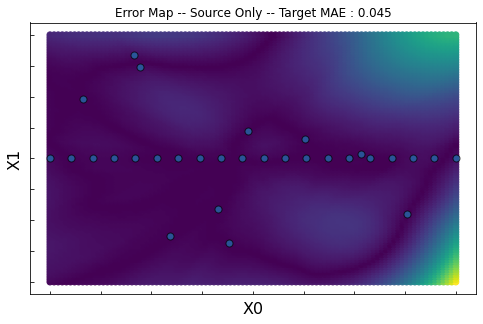
Source Only

np.random.seed(0)
tf.random.set_seed(0)
estimator = clone_model(model)
estimator.compile(loss="mse", optimizer=Adam(0.001))
estimator.fit(Xs, ys, **fit_params);

yp_grid = estimator.predict(np.stack([x_grid.ravel(), y_grid.ravel()], -1)).ravel()
error_grid = np.abs(yp_grid-z_grid)

score = mean_absolute_error(
    estimator.predict(Xt).ravel(), yt)

fig, ax = plt.subplots(1, 1, figsize=(8, 5))

ax.plot(Xs[:, 0], Xs[:, 1], '.', c="C0", ms=14, alpha=0.7, markeredgecolor="black")
ax.scatter(x_grid.ravel(), y_grid.ravel(), c=error_grid)

ax.set_xlabel("X0", fontsize=16)
ax.set_ylabel("X1", fontsize=16)
ax.set_title("Error Map -- Source Only -- Target MAE : %.3f"%score)

ax.set_yticklabels([])
ax.set_xticklabels([])
ax.tick_params(direction ='in')

plt.show()

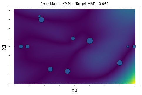
KMM

np.random.seed(0)
kmm = KMM(model, gamma=2., random_state=0)
kmm.fit(Xs, ys, Xt, **fit_params);

Fit weights...
     pcost       dcost       gap    pres   dres
 0:  2.7084e+04 -4.3392e+05  1e+07  6e-01  2e-14
 1:  2.3438e+02 -1.0551e+05  2e+05  4e-03  2e-11
 2:  1.7072e+02 -2.1481e+04  2e+04  9e-06  2e-12
 3:  1.6458e+02 -8.2292e+02  1e+03  4e-07  5e-14
 4:  1.0422e+02 -6.2452e+02  7e+02  2e-07  3e-14
 5: -7.2423e+01 -9.3040e+02  9e+02  5e-08  6e-15
 6: -7.7015e+01 -2.8294e+02  2e+02  1e-08  2e-15
 7: -7.9350e+01 -2.8047e+02  2e+02  1e-08  1e-15
 8: -8.7166e+01 -1.2479e+02  4e+01  2e-16  3e-16
 9: -8.9553e+01 -9.7350e+01  8e+00  2e-16  1e-16
10: -9.0635e+01 -9.2636e+01  2e+00  2e-16  2e-16
11: -9.1022e+01 -9.1316e+01  3e-01  2e-16  1e-16
12: -9.1106e+01 -9.1145e+01  4e-02  2e-16  1e-16
13: -9.1116e+01 -9.1120e+01  4e-03  2e-16  2e-16
14: -9.1118e+01 -9.1118e+01  6e-05  2e-16  2e-16
Optimal solution found.
Fit Estimator...

yp_grid = kmm.predict(np.stack([x_grid.ravel(), y_grid.ravel()], -1)).ravel()
error_grid = np.abs(yp_grid-z_grid)

score = mean_absolute_error(
    kmm.predict(Xt).ravel(), yt)

weights = kmm.predict_weights() * 100

fig, ax = plt.subplots(1, 1, figsize=(8, 5))

ax.scatter(x_grid.ravel(), y_grid.ravel(), c=error_grid)
ax.scatter(Xs[:, 0], Xs[:, 1], c="C0", s=weights, alpha=0.7, edgecolor="black")

ax.set_xlabel("X0", fontsize=16)
ax.set_ylabel("X1", fontsize=16)
ax.set_title("Error Map -- KMM -- Target MAE : %.3f"%score)

ax.set_yticklabels([])
ax.set_xticklabels([])
ax.tick_params(direction ='in')

plt.show()

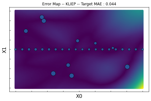
KLIEP

np.random.seed(0)
kliep = KLIEP(model, sigmas=[0.001, 0.01, 0.1, 0.5, 1., 2., 5., 10.], random_state=0, max_centers=200)
kliep.fit(Xs, ys, Xt, **fit_params);

Fit weights...
Cross Validation process...
Parameter sigma = 0.0010 -- J-score = -0.000 (0.000)
Parameter sigma = 0.0100 -- J-score = -0.004 (0.001)
Parameter sigma = 0.1000 -- J-score = -0.033 (0.009)
Parameter sigma = 0.5000 -- J-score = -0.068 (0.019)
Parameter sigma = 1.0000 -- J-score = -0.002 (0.022)
Parameter sigma = 2.0000 -- J-score = 0.157 (0.026)
Parameter sigma = 5.0000 -- J-score = 0.393 (0.023)
Parameter sigma = 10.0000 -- J-score = 0.467 (0.008)
Fit Estimator...

yp_grid = kliep.predict(np.stack([x_grid.ravel(), y_grid.ravel()], -1)).ravel()
error_grid = np.abs(yp_grid-z_grid)

score = mean_absolute_error(
    kliep.predict(Xt).ravel(), yt)

weights = kliep.predict_weights() * 100

fig, ax = plt.subplots(1, 1, figsize=(8, 5))

ax.scatter(x_grid.ravel(), y_grid.ravel(), c=error_grid)
ax.scatter(Xs[:, 0], Xs[:, 1], c="C0", s=weights, alpha=0.7, edgecolor="black")

ax.set_xlabel("X0", fontsize=16)
ax.set_ylabel("X1", fontsize=16)
ax.set_title("Error Map -- KLIEP -- Target MAE : %.3f"%score)

ax.set_yticklabels([])
ax.set_xticklabels([])
ax.tick_params(direction ='in')

plt.show()