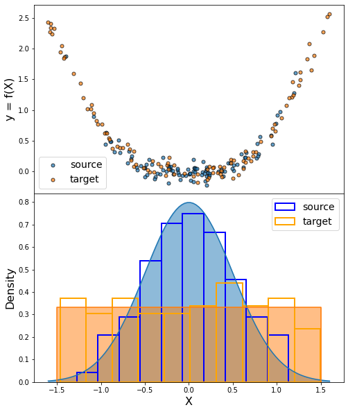
Sample Bias 1D

Run in Google Colab

View on GitHub

The following example is a 1D regression domain adaptation issue. The goal is to learn the regression task on the target data (orange points) knowing only the labels on the source data (blue points).

In this example, there is a sample bias between the source and target datasets. The sources are drawn according to a gaussian distribution whereas the targets are uniformly distributed.

The following methods are being tested:

• Source Only

• KMM

• KLIEP

import numpy as np
import matplotlib.pyplot as plt
import matplotlib.animation as animation
from sklearn.neural_network import MLPRegressor
from sklearn.metrics import mean_absolute_error, mean_squared_error
from sklearn.metrics.pairwise import rbf_kernel
from adapt.instance_based import KMM, KLIEP

Setup

def f(x, noise=0.1):
    return (x ** 4) * np.exp(-x**2) + (x**2) * (1 - np.exp(-x**2)) + noise * np.random.randn(len(x))

def gaussian(x, s=0.5):
    return 1./np.sqrt( 2. * np.pi * s**2 ) * np.exp( -x**2 / ( 2. * s**2 ) )

np.random.seed(0)
lin = np.linspace(-1.6, 1.6, 100)
Xs = np.random.randn(100) * 0.5
Xt = np.random.random(100) * 3 - 1.5
ys = f(Xs)
yt = f(Xt)

fig, (ax1, ax2) = plt.subplots(2, 1, figsize=(8, 10))

ax1.plot(Xs, ys, '.', label="source", ms=10, alpha=0.7, markeredgecolor="black")
ax1.plot(Xt, yt, '.', label="target", ms=10, alpha=0.7, markeredgecolor="black")
ax2.hist(Xs, density=True, edgecolor='blue', label="source", fc=(0., 0, 0, 0.), lw=2)
ax2.hist(Xt, density=True, edgecolor='orange', label="target", fc=(0., 0, 0, 0.), lw=2)
ax2.plot(lin, gaussian(lin), color="C0")
ax2.fill_between(lin, gaussian(lin), alpha=0.5, color="C0")
ax2.plot([-1.5, -1.5, 1.5, 1.5], [0, 1/3., 1/3., 0.], color="C1")
ax2.fill_between([-1.5, -1.5, 1.5, 1.5], [0, 1/3., 1/3., 0.], alpha=0.5, color="C1")

ax1.legend(fontsize=14)
ax2.legend(fontsize=14)

ax2.set_xlabel("X", fontsize=16)

ax1.set_ylabel("y = f(X)", fontsize=16)
ax2.set_ylabel("Density", fontsize=16)

plt.subplots_adjust(hspace=0.)

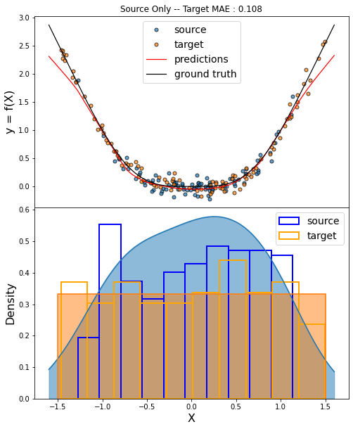
Source Only

np.random.seed(0)
estimator = MLPRegressor((100, 100))
estimator.fit(Xs.reshape(-1,1), f(Xs));

yp_lin = estimator.predict(lin.reshape(-1, 1))

score = mean_absolute_error(estimator.predict(Xt.reshape(-1, 1)).ravel(), yt)

fig, ax = plt.subplots(1, 1, figsize=(8, 5))

ax.plot(Xs, ys, '.', label="source", ms=10, alpha=0.7, markeredgecolor="black")
ax.plot(Xt, yt, '.', label="target", ms=10, alpha=0.7, markeredgecolor="black")
ax.plot(lin, yp_lin, label="predictions", lw=1.2, color="red")
ax.plot(lin, f(lin, 0), label="ground truth", lw=1.2, color="black")

ax.legend(fontsize=14)
ax.set_xlabel("X", fontsize=16)
ax.set_ylabel("y = f(X)", fontsize=16)
ax.set_title("Source Only -- Target MAE : %.3f"%score)

plt.show()

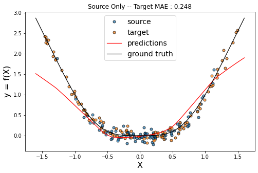
KMM

np.random.seed(0)
estimator = MLPRegressor((100, 100))
kmm = KMM(estimator, gamma=0.1, random_state=0)
kmm.fit(Xs.reshape(-1,1), ys, Xt.reshape(-1,1));

Fit weights...
     pcost       dcost       gap    pres   dres
 0:  4.7447e+04 -7.7223e+05  3e+07  4e-01  2e-15
 1: -1.3351e+02 -2.6366e+05  3e+05  1e-03  5e-13
 2: -1.8642e+02 -2.0333e+04  2e+04  2e-05  1e-14
 3: -4.7934e+02 -1.8983e+04  2e+04  1e-05  1e-14
 4: -4.3560e+03 -2.3704e+04  2e+04  3e-16  4e-16
 5: -4.3665e+03 -4.9080e+03  5e+02  2e-16  2e-16
 6: -4.3757e+03 -4.5211e+03  1e+02  2e-16  1e-16
 7: -4.3851e+03 -4.4686e+03  8e+01  1e-16  1e-16
 8: -4.3854e+03 -4.3884e+03  3e+00  2e-16  1e-16
 9: -4.3854e+03 -4.3855e+03  4e-02  2e-16  2e-16
10: -4.3854e+03 -4.3854e+03  2e-03  1e-16  1e-16
Optimal solution found.
Fit Estimator...

np.random.seed(0)
yp_lin = kmm.predict(lin.reshape(-1, 1))
score = mean_absolute_error(kmm.predict(Xt.reshape(-1, 1)).ravel(), yt)

weights = kmm.predict_weights()
Xs_weighted = np.random.choice(Xs, 3 * len(Xs), p=weights / weights.sum())
kde = rbf_kernel(lin.reshape(-1, 1), Xs_weighted.reshape(-1,1), gamma=3.).sum(1)
kde /= kde.sum()
kde *= 40.

fig, (ax1, ax2) = plt.subplots(2, 1, figsize=(8, 10))

ax1.plot(Xs, ys, '.', label="source", ms=10, alpha=0.7, markeredgecolor="black")
ax1.plot(Xt, yt, '.', label="target", ms=10, alpha=0.7, markeredgecolor="black")
ax1.plot(lin, yp_lin, label="predictions", lw=1.2, color="red")
ax1.plot(lin, f(lin, 0), label="ground truth", lw=1.2, color="black")

ax2.hist(Xs_weighted, density=True, edgecolor='blue', label="source", fc=(0., 0, 0, 0.), lw=2)
ax2.hist(Xt, density=True, edgecolor='orange', label="target", fc=(0., 0, 0, 0.), lw=2)
ax2.plot(lin, kde, color="C0")
ax2.fill_between(lin, kde, alpha=0.5, color="C0")
ax2.plot([-1.5, -1.5, 1.5, 1.5], [0, 1/3., 1/3., 0.], color="C1")
ax2.fill_between([-1.5, -1.5, 1.5, 1.5], [0, 1/3., 1/3., 0.], alpha=0.5, color="C1")

ax1.legend(fontsize=14)
ax2.legend(fontsize=14)

ax2.set_xlabel("X", fontsize=16)

ax1.set_ylabel("y = f(X)", fontsize=16)
ax2.set_ylabel("Density", fontsize=16)

plt.subplots_adjust(hspace=0.)

ax1.set_title("Source Only -- Target MAE : %.3f"%score)

plt.show()

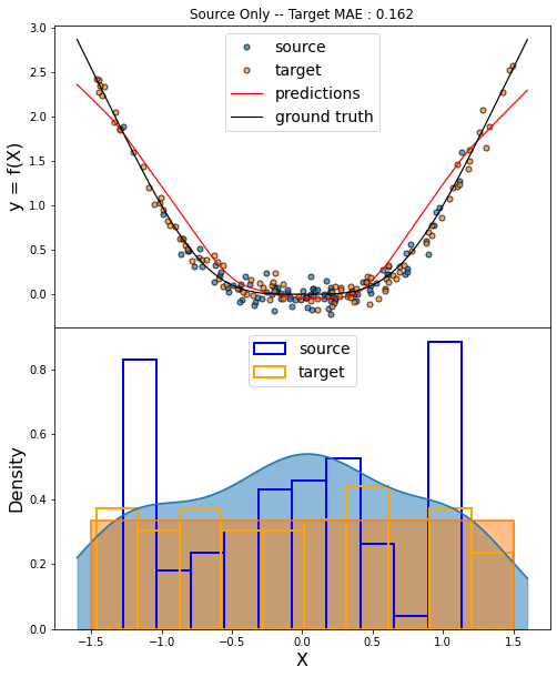
KLIEP

np.random.seed(0)
estimator = MLPRegressor((100, 100))
kliep = KLIEP(estimator, sigmas=[0.001, 0.01, 0.1, 0.5, 1., 2., 5.], random_state=0)
kliep.fit(Xs.reshape(-1,1), ys, Xt.reshape(-1,1));

Fit weights...
Cross Validation process...
Parameter sigma = 0.0010 -- J-score = -0.000 (0.000)
Parameter sigma = 0.0100 -- J-score = -0.005 (0.002)
Parameter sigma = 0.1000 -- J-score = -0.044 (0.015)
Parameter sigma = 0.5000 -- J-score = 0.003 (0.011)
Parameter sigma = 1.0000 -- J-score = 0.114 (0.014)
Parameter sigma = 2.0000 -- J-score = 0.236 (0.035)
Parameter sigma = 5.0000 -- J-score = 0.349 (0.090)
Fit Estimator...

np.random.seed(0)
yp_lin = kliep.predict(lin.reshape(-1, 1))
score = mean_absolute_error(kliep.predict(Xt.reshape(-1, 1)).ravel(), yt)

weights = kliep.predict_weights()
Xs_weighted = np.random.choice(Xs, 3 * len(Xs), p=weights / weights.sum())
kde = rbf_kernel(lin.reshape(-1, 1), Xs_weighted.reshape(-1,1), gamma=3.).sum(1)
kde /= kde.sum()
kde *= 40.

fig, (ax1, ax2) = plt.subplots(2, 1, figsize=(8, 10))

ax1.plot(Xs, ys, '.', label="source", ms=10, alpha=0.7, markeredgecolor="black")
ax1.plot(Xt, yt, '.', label="target", ms=10, alpha=0.7, markeredgecolor="black")
ax1.plot(lin, yp_lin, label="predictions", lw=1.2, color="red")
ax1.plot(lin, f(lin, 0), label="ground truth", lw=1.2, color="black")

ax2.hist(Xs_weighted, density=True, edgecolor='blue', label="source", fc=(0., 0, 0, 0.), lw=2)
ax2.hist(Xt, density=True, edgecolor='orange', label="target", fc=(0., 0, 0, 0.), lw=2)
ax2.plot(lin, kde, color="C0")
ax2.fill_between(lin, kde, alpha=0.5, color="C0")
ax2.plot([-1.5, -1.5, 1.5, 1.5], [0, 1/3., 1/3., 0.], color="C1")
ax2.fill_between([-1.5, -1.5, 1.5, 1.5], [0, 1/3., 1/3., 0.], alpha=0.5, color="C1")

ax1.legend(fontsize=14)
ax2.legend(fontsize=14)

ax2.set_xlabel("X", fontsize=16)

ax1.set_ylabel("y = f(X)", fontsize=16)
ax2.set_ylabel("Density", fontsize=16)

plt.subplots_adjust(hspace=0.)

ax1.set_title("Source Only -- Target MAE : %.3f"%score)

plt.show()